Efficient Source Selection for Federated SPARQL Queries using Adjacent Predicate Information
Yudai Ogura [1], Tadashi Masuda [2], and Toshiyuki Amagasa [2]
- Graduate School of Science and Technology University of Tsukuba, Japan
- Center for Computational Sciences, University of Tsukuba, Japan
Abstract
With the growing adoption of Linked Open Data (LOD), many distributed knowledge bases have been developed using the RDF format. These knowledge bases each have unique characteristics, and querying across them can reveal richer and more comprehensive insights. To support such cross-repository querying,federated RDF query processing is essential. However, the performance of federated query execution largely depends on efficient source selection — the process of identifying which data sources are relevant to a given query. In this paper, we propose a novel source selection method for federated RDF queries based on a new summarization technique. Our approach precomputes the existence of shared elements between predicate pairs within each data source, considering three types of join patterns: subject–subject, subject–object, and object–object. These relationships are stored in a matrix-form summary for each data source. During query execution, our method identifies predicate pairs from triple patterns that share join keys within a basic graph pattern (BGP) and uses the precomputed summaries to efficiently determine the relevant data sources. Experimental results on the FedBench benchmark show that our method improves the efficiency of source selection and significantly reduces overall query execution time.
- Keywords: RDF· Knowledge base· Federated RDF query· Summary
1 Introduction
The rapid growth of Linked Open Data (LOD) has made hundreds of interconnected knowledge bases—accessible via SPARQL endpoints—available on the web. While this opens up new possibilities for data integration and knowledge discovery, executing SPARQL queries across these large-scale, distributed data sources remains a significant challenge. One of the key difficulties lies in identifying the relevant data sources needed to answer a given query efficiently.
Most existing approaches to federated RDF query processing rely on triple pattern-wise source selection (TPWSS), where candidate sources are selected independently for each triple pattern in the query [2,13,10]. However, this strategy often results in the inclusion of sources that produce intermediate results irrelevant to the final answer. This not only increases network traffic but also degrades overall query performance.
To address this, HiBISCuS [9] introduced a join-aware source selection strategy that summarizes data sources based on the authority part (i.e., the domain name) of subject and object URIs associated with each predicate. At query time, HiBISCuS selects sources only if their predicates share common authorities in join positions. While effective in filtering out clearly irrelevant sources, this method cannot distinguish between multiple sources that use the same URI authority. As a result, it often selects more sources than necessary. Some extended versions of HiBISCuS attempt to improve accuracy by storing full URI strings in the summaries. However, these enhancements come at the cost of reduced compression and higher computation due to expensive string matching operations, ultimately harming performance [4].
In this paper, we propose a novel source selection method called MAPS (Matrix-format Adjacent Predicates Summary), which overcomes these limitations by leveraging adjacent predicates within the data. Our method begins by extracting all predicates from a given set of data sources and generating all possible predicate pairs. For each pair, we precompute whether the pair shares common elements under different join patterns—subject–subject, subject–object, and object–object—and store the results in a matrix-form summary.
At query time, we identify predicate pairs between triple patterns that share a join key within a basic graph pattern (BGP) and use the corresponding MAPS to determine the relevant data sources. This matrix-based representation enables both high compression and fast lookups, avoiding costly string comparisons while improving the precision of source selection.
To validate the effectiveness of our approach, we conducted a comprehensive evaluation comparing MAPS with existing techniques. We assessed performance across five key metrics: source selection time, number of selected sources, numberof SPARQL ASK queries issued during source selection, overall query execution time, and summary generation time/compression ratio. The results demonstrate that our method outperforms existing approaches in both accuracy and efficiency.
2 Preliminaries
2.1 k2-Tree
k2-Tree [1] is a compression technique for storing large sparse matrices by recursively partitioning the matrix and recording only the regions containing information using a tree structure. This approach significantly reduces storage requirements while maintaining efficient access to the data. The transformation into a tree structure follows these steps:
- The entire adjacency matrix is divided into k × k blocks.
- If a block contains at least one 1, it is stored as a node in the tree structure and further subdivided.
- Blocks containing only 0s are not subdivided and are instead stored as a single 0 node.
- This recursive partitioning continues until the entire matrix is represented as a tree structure.
The k2-Tree is stored using the following two bit sequences:
- – T (Tree bit sequence): Records all nodes except the leaves in breadth-first order (BFS). If a block contains at least one 1, a 1 is stored; otherwise, a 0 is stored.
- – L (Leaf bit sequence): Stores the actual data of the original adjacency matrix at the leaf level of the tree, containing either 1 or 0.
2.2 Definitions
An RDF resource is identified using a Uniform Resource Identifier (URI). Each URI consists of multiple components: scheme, authority, path, query, and fragment. In this paper, we collectively refer to the scheme and authority components as authority.
For the following discussion, we use an example where a query in Figure 2 is executed against the data sources shown in Figure 1.
Definition 1 (Relevant Source Set) A data source \(d ∈ D\) is considered relevant to a triple pattern \(tp_i ∈T P\) if at least one triple contained in d matches \(tp_i\). The relevant source set \(R_i ⊆ D\) for a triple pattern tpi consists of all data sources that are relevant to that specific triple pattern. For example, in Figure 2, the relevant source set for \(tp_2\) is {DBpedia, MusicBrainz, LMDB}.
However, a relevant source does not necessarily contribute to the final result set of query \(q\). This is because the results obtained from a certain source \(d\) for a triple pattern \(tp_i\) may be filtered out when performing joins with results from other triple patterns in query \(q\).
Definition 2 (Optimal Source Set) The optimal source set \(O_i ⊆ R_i\) for a triple pattern \(tp_i ∈ T P\) consists of only those relevant sources \(d ∈ R_i\) that actually contribute to computing the complete query result set. For example, in Figure 2, the optimal source set for \(tp_2\) is {MusicBrainz}.
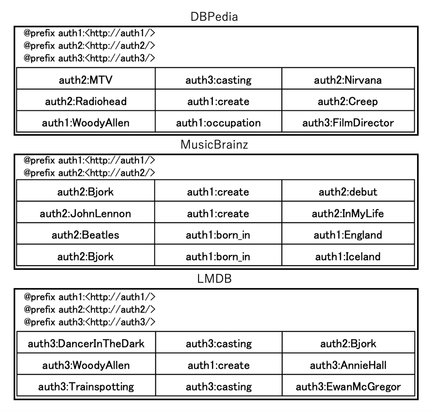
Fig.1: Data Sources
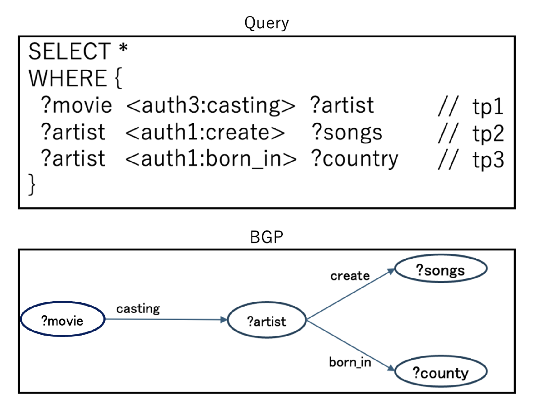
Fig.2: SPARQL Query and Its BGP
3 Related Work
Information source selection methods for federated RDF queries can be classified into three categories: summary-based source selection methods, non-summary-based source selection methods, and hybrid source selection methods [8].
Summary-based source selection methods include approaches such as DARQ [6] and ADERIS [3], which rely solely on summaries for source selection. This generally results in high-speed execution. However, since these methods perform source selection based only on predicates without considering the subjects or objects of each triple pattern, their selection accuracy may be inferior [8].
Non-summary-based source selection methods include approaches such as FedX [13]. These methods do not use pre-stored summaries and instead select sources based on the latest data at all times. The source selection algorithm is executed using SPARQL ASK queries, which match not only predicates but also subjects and objects. This makes them more efficient than summary-based methods [8]. However, the increased number of SPARQL ASK queries may lead to longer query execution times [8].
Hybrid source selection methods combine the two approaches mentioned above, utilizing both summaries and SPARQL ASK queries for source selection. Well-known examples include DAW [10], TopFed [11], and SPLENDID [2]. These methods perform source selection based on fixed values within each triple pattern. For example, in the query example shown in Figure 2, tp1 has the fixed predicate auth3:casting, tp2 has auth1:create, and tp3 has auth1:born_in. Selecting sources based on these fixed values for each triple pattern results in tp1 being assigned to {DBPedia, LMDB}, tp2 to {DBPedia, MusicBrainz, LMDB}, and tp3 to {MusicBrainz}. However, since these methods do not consider joins between triple patterns at the source selection stage, intermediate results may be retrieved from sources that do not contribute to the final results, potentially increasing execution time.
To address this issue, HiBISCuS [9] itroduced a source selection method that considers joins between triple patterns. Specifically, it records the domain part (referred to as the “authority”) of the subject and object URIs for all predicates present in the target sources as summaries. During source selection, it identifies common authorities for join keys based on pre-generated summaries, thereby excluding sources that do not contribute to the final results.
For example, in the query shown in Figure 2, the common authority among the object of auth3:casting, the subject of auth1:create, and the subject of auth1:born_in is
Furthermore, methods such as TBSS [7] and SemCat [4] have been developed as extensions of the HiBISCuS summary format. These methods retain the string following the authority in URIs, thereby improving the accuracy of source selection. However, they suffer from trade-offs, such as lower summary compression rates and increased computational costs due to string matching, which can degrade performance. While these methods enhance source selection accuracy by extending the HiBISCuS summary format, they do not completely eliminate the selection of sources that do not contribute to the final results.
In this study, we propose a new source selection method for efficient federated RDF querying. Instead of using the HiBISCuS summary format, our approach records precomputed results in a matrix as a novel summarization technique for source selection.
4 Proposed Method
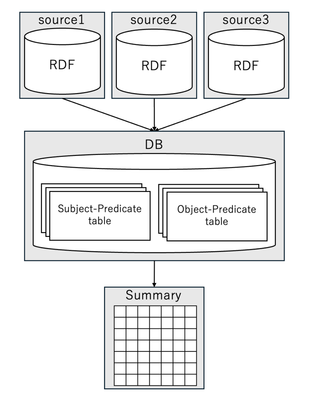
Fig.3: Overall process of summary creation
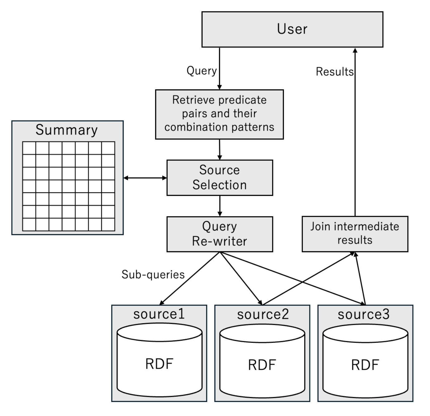
Fig.4: Overview of the query process
In this study, we propose a method for efficiently performing federated RDF queries by pre-generating summaries and selecting information sources based on these summaries during query processing. This approach resolves the trade-off between source selection accuracy and execution time/compression rate, which previous URI string-matching-based source selection methods such as HiBISCuS [9], TBSS [7], and SemCat [4] faced due to the need to retain a large number of characters in the summary.
Section 4.1 describes the types of summaries generated by our method, Section 4.2 explains the summary generation process, and Section 4.3 details the source selection method.
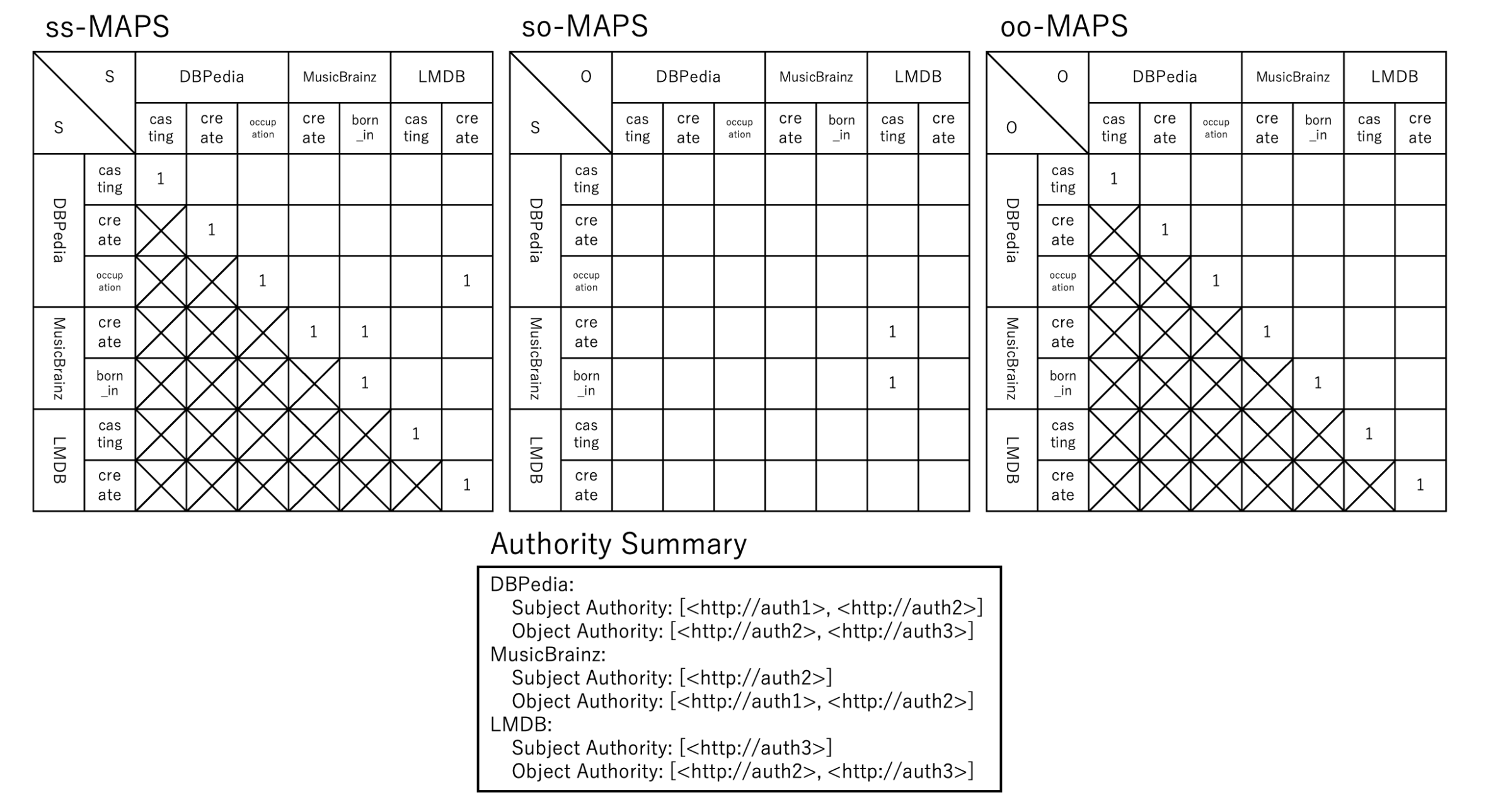
Fig.5: Summary
4.1 Types of Summaries
Our method generates three types of summaries: ss (subject-subject)-MAPS, so (subject-object)-MAPS, and oo (object-object)-MAPS. Figure 5 shows the summaries generated for the set of information sources depicted in Figure 1.
MAPS (Matrix format Adjacent Predicates Summary)
- ss-MAPS: This summary stores whether the subjects of paired predicates share common elements (hereafter referred to as “ss-common”).
- so-MAPS: This summary stores whether the subject of one predicate and the object of another share common elements (hereafter referred to as “so-common”).
- oo-MAPS: This summary stores whether the objects of paired predicates share common elements (hereafter referred to as “oo-common”).
Authority Summary This summary stores the set of authorities of subjects and the set of authorities of objects that exist in each dataset.
4.2 Summary Generation
This section explains the method for generating summaries. The overall process of Matrix format Summary (MAPS) generation is illustrated in Figure 3.
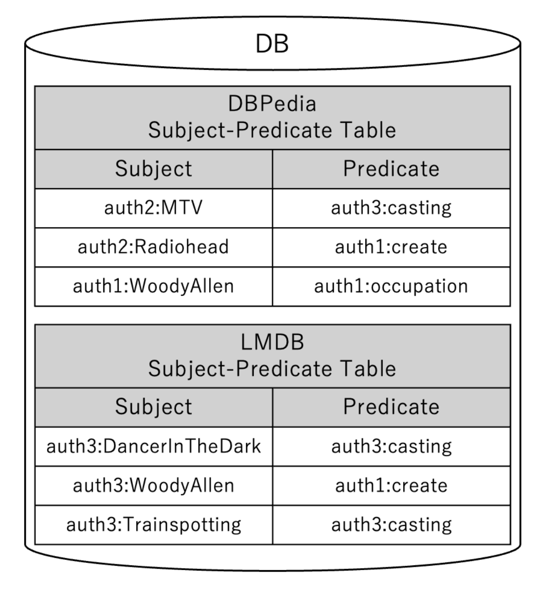
Fig.6: Database for generating summaries
Algorithm 1 Database Creation Algorithm
Require: datasources D // list of available datasources
1: for each pair ∈ predicatesPairs do
2:      SbjPrd= fetchSbjPrd(D)
3:      ObjPrd= fetchObjPrd(D)
4:      registerTable(SbjPrd)
5:      registerTable(ObjPrd)
6: end for
First, the data required for summary generation is stored in a local database from the information sources. Then, MAPS is generated using the data stored in the database. Additionally, simplified code for each process is provided in Algorithm 1 and Algorithm 2.
The method for creating the database is explained in detail according to Algorithm 1. First, from each information source, the pairs of “subject and predicate” and “object and predicate” are retrieved (lines 2–3). Then, the retrieved data is registered in the database as Subject-Predicate Tables and Object-Predicate Tables (lines 4–5). For example, when creating the database shown in Figure 6 from the information sources in Figure 1, the Subject-Predicate Tables from DBPedia and LMDB are stored. This process reduces the number of accesses to large-scale information sources. Additionally, since only the data necessary for MAPS generation is extracted, computational costs are reduced.
Next, the method for generating MAPS is explained in detail according to Algorithm 2. First, all pairs of target information sources are retrieved (line 1). Then, for each pair of information sources, the Subject-Predicate Tables and Object-Predicate Tables are retrieved (lines 5–8). For ss-common predicate pairs, the Subject-Predicate Tables from both information sources are joined using the subject as the join key (line 9).
For so-common predicate pairs, the Subject-Predicate Table from one source and the Object-Predicate Table from the other are joined using the subject and object as the join keys (lines 10–11). For oo-common predicate pairs, the Object-Predicate Tables from both information sources are joined using the object as the join key (line 12). For example, when generating MAPS from the database in Figure 6, the Subject-Predicate Tables from DBPedia and LMDB are joined using the subject as the join key. As a result, the predicate pair (auth1:occupation, auth1:create) is identified as an ss-common predicate pair and stored in MAPS.
Since ss-MAPS and oo-MAPS form symmetric matrices, it is unnecessary to swap the left and right tables when retrieving join results. However, for so-MAPS, the left and right tables must be swapped to obtain the join results. This is because the relationship depends on whether the subject and object used as join keys correspond to the respective predicates in the predicate pair.
Algorithm 3 presents the overall algorithm for Authority Summary generation. This algorithm extracts all subject authorities and object authorities from the target information sources.
Finally, since the matrices representing each join pattern are expected to be sparse, only the row index and column index pairs of nonzero elements are stored when saving the summary.
Algorithm 2 Summary Generation Algorithm
Require: datasources D // list of available datasources
1: DPairs= extractDPairs(D)
2: for each pair ∈ DPairs do
3:      d1 = Pair[0]
4:      d2 = Pair[1]
5:      SP d1 = fetchSbjPrdFromDB(d1)
6:      SP d2 = fetchSbjPrdFromDB(d2)
7:      OP d1 = fetchObjPrdFromDB(d1)
8:      OP d2 = fetchObjPrdFromDB(d2)
9:      ssPairs= SPd1 INNER JOIN SPd2 ON sbj
10:     soPairs= SPd1 INNER JOIN OPd2 ON [sbj, obj]
11:     osPairs= OPd1 INNER JOIN SPd2 ON [obj, sbj]
12:     ooPairs= OPd1 INNER JOIN OPd2 ON obj
13: end for
Algorithm 3 Authority Summary Generation Algorithm
Require: datasources D // list of available datasources
1: for each di ∈ D do
2:      sbjAuthList= extractSbjAuthList(di)
3:      objAuthList= extractObjAuthList(di)
4: end for
4.3 Query Processing
The overall query process is illustrated in Figure 4. When a query is received, the system first references the summary and selects the data sources to be accessed. Then, the query is rewritten to match the federated RDF query processing. Finally, the rewritten query is executed to obtain the results.
Algorithm 4 Source Selection Algorithm
Require: SM //MAPS; SA//Authority Summary; Q//query
1: triples= extractTriples(Q)
2: R= initializeTripleDatasetDict(triples)
3: joinTriplePairs= extractJoinTriplePairs(triples)
4: for each pair ∈ joinTriplePairs do
5:      R = updateDict(R, pair, SM , SA)
6: end for
7: for each triple ∈ triples do
8:      s, p, o = triple
9:      Rtpi = R.get(triple)
10:     I= Rtpi.get(1)
11:     for each dset ∈ Rtpi do
12:         I= I ∩ dset
13:         if size(I) > 1 and (bound(s) or bound(o)) then
14:             label = ASK(s, p, o, I)
15:         end if
16:     end for
17: end for
The following sections explain the method for selecting the data sources to be accessed. Algorithm 4 presents the source selection algorithm.
The source selection process based on the summary for the given query is performed in the following steps. At the end of each step, an example explanation is provided using the query shown in Figure 2.
-
Initialize the variable R to store relevant data sources for each triple (line 2).
ex)
R={tp1:{}, tp2:{}, tp3:{}}
-
Obtain pairs of triple patterns based on join keys (line 3).
ex)
The join key is ?artist, and by using ?artist as the basis, three pairs are obtained: {(tp1, tp2), (tp1, tp3), (tp2, tp3)}.
-
Extract the predicate pairs and join patterns for each paired triple pattern. Query the corresponding MAPS for the extracted predicate pairs to check if results exist for the given join pattern, and add the results to R (lines 4–6). Additionally, if the subject or object is specified, use the authority summary for further refinement.
ex)
(tp1, tp2) Pair:
The predicate pair is (auth3:casting, auth1:create), and the join pattern is object–subject. In this case, the order is swapped to subject–object, and a query is performed on so-MAPS for the following pairs:
[(DBPedia:create, DBPedia:casting), (DBPedia:create, LMDB:casting), (MusicBrainz:create, DBPedia:casting), (MusicBrainz:create, LMDB:casting), (LMDB:create, DBPedia:casting), (LMDB:create, LMDB:casting)]
The matching pair found is (MusicBrainz:create, LMDB:casting).
R={tp1:{{LMDB}}, tp2:{{MusicBrainz}}, tp3:{}}
(tp1, tp3) Pair:
The predicate pair is (auth3:casting, auth1:born_in), and the join pattern is object-subject. Again, the order is swapped to subject-object, and a query is performed on so-MAPS for the following pairs:
[(MusicBrainz:born_in, DBPedia:casting), (MusicBrainz:born_in, LMDB:casting)]
The matching pair found is (MusicBrainz:born_in, LMDB:casting).
R={tp1:{{LMDB},{LMDB}}, tp2:{{MusicBrainz}},
tp3:{{MusicBrainz}}}
(tp2, tp3) Pair: The predicate pair is (auth1:create, auth1:born_in), and the join pattern is subject-subject.A query is performed on ss-MAPS for the following pairs:
[(DBPedia:create, MusicBrainz:born_in), (MusicBrainz:create, MusicBrainz:born_in), (LMDB:create, MusicBrainz:born_in)]
The matching pair found is (MusicBrainz:create, MusicBrainz:born_in).
R={tp1:{{LMDB},{LMDB}}, tp2:{{MusicBrainz}, {MusicBrainz}}, tp3:{{MusicBrainz}, {MusicBrainz}}}
-
Obtain the common data sources for each triple pattern.Furthermore, if the subject or object is specified and additional refinement is possible, use SPARQL ASK queries to further filter the data sources. The final set of selected data sources is determined based on these results.
ex)
The following shows the collection of candidate sets for each triple pattern and the computation of their common data sources:
Itp1={LMDB}, Itp2={MusicBrainz}, Itp3={MusicBrainz}
The above operations do not compromise recall. This is because the join operations are processed in a manner similar to a logical “AND”, meaning that any data retrieved for part of the query must also be joinable with other parts; otherwise, it will not contribute to the final results.
5 Experiment
In this chapter, we present the results of our performance evaluation of the proposed method by comparing it with a baseline approach using nine datasets and multiple evaluation metrics. As a baseline method, we use HiBISCuS [9]. Additionally, we conducted experiments using NumPy’s ndarray and k2-Tree as data structures for storing MAPS. Furthermore, the memory usage of each data structure is reported in Table 4.
For evaluation, we utilized FedBench [12], which is widely used for evaluating federated RDF queries [9,7,5,2,8,10]. The nine information sources from FedBench were uploaded to a Fuseki server for testing.
The proposed method is evaluated based on the following five performance metrics:
– Number of selected data sources
– Total number of SPARQL ASK queries
– Execution time of source selection
– Query execution time
– Summary generation time/compression rate
The results are presented in Table 2. The reported values for source selection execution time and query execution time are the average of five measurements.
5.1 Experimental Environment
All experiments were conducted in the environment described in Table 1. The proposed method was implemented using Python 3.8.19. For consistency, the baseline method was also re-implemented in Python 3.8.19.
| OS | Ubuntu 24.04 LTS |
| CPU | Intel Core i7-13700 |
| RAM | 32GB |
| Programming Language | Python 3.8.19 |
5.2 Experimental Results
The experimental results are summarized in Table 2. Bold values indicate cases where the proposed method outperforms HiBISCuS. Underlined values indicate cases where the performance difference between storing MAPS in NumPy’s ndarray and k2-Tree is notable.
Number of Selected Data Sources The number of selected data sources refers to the total number of datasets selected for querying for each triple pattern. The results are shown in the SSN column of Table 2. In CD1, CD2, CD3, CD4, CD5, and LS4, no improvement was observed, and the selection was the same as HiBISCuS. However, in LS2, LS5, and LS7, the number of selected sources was reduced, demonstrating the effectiveness of the proposed method.
Total Number of SPARQL ASK Queries The total number of SPARQL ASK queries refers to the total number of queries sent during the source selection process. The results are shown in the AN column of Table 2.
For CD3, CD4, CD5, LS4, LS5, and LS7, HiBISCuS already did not send any SPARQL ASK queries, so the results remained the same. However, in CD1, CD2, and LS2, where HiBISCuS did send SPARQL ASK queries, the proposed method reduced the number of SPARQL ASK queries by 11, 9, and 16 in CD1, CD2, and LS2 respectively, thereby enhancing efficiency.
Source Selection Execution Time The execution time for source selection is measured as the time taken from receiving a query to selecting the relevant data sources using the summaries. The results are shown in the SST column of Table 2. For queries where the number of SPARQL ASK queries was 0, using NumPy-based MAPS, the proposed method achieved an average speed-up of 270x and a maximum speed-up of 500x, demonstrating significant improvements. For queries where SPARQL ASK queries were still required, using k2-Tree-based MAPS, LS2 saw a 53x speed-up, and CD1 was 2.7x faster.
Query Execution Time Query execution time is measured as the time taken from sending the query to the endpoint until the result set is received. The results are shown in the QET column of Table 2. For queries where no improvement in source selection was observed (CD1, CD2, CD3, CD4, CD5, LS4), the difference in query execution time was within the margin of error, and no significant improvement was observed. For queries where source selection was improved (LS2, LS5, LS7), execution time was also significantly improved. In LS5, HiBISCuS exceeded the execution time limit and failed to return a result, whereas the proposed method successfully returned a result in 6148 ms. In LS7, query execution time was reduced from 11738 ms to 2759 ms, demonstrating substantial improvement.
Summary Generation Time and Compression Rate The summary generation time and compression rate are shown in Table 3. Summary generation time was reduced by approximately 20 minutes compared to HiBISCuS. Compression rate was 0.2% lower than HiBISCuS but remained highly efficient overall.
SSN: Number of selected data sources, AN: Number of SPARQL ASK queries, SST: Source selection time (ms), QET: Query execution time (ms).
| |HiBISCuS | |Proposed Method(NumPy) | |Proposed Method(k2-Tree) |
|---|
| Query | SSN | AN | SST | QET | SSN | AN | SST | QET | SSN | AN | SST | QET |
|---|---|---|---|---|---|---|---|---|---|---|---|---|
| CD1 | 4 | 18 | 103.66 | 115 | 4 | 7 | 60.38 | 87 | 4 | 7 | 37.89 | 83 |
| CD2 | 3 | 9 | 34.87 | 12 | 3 | 0 | 0.16 | 12 | 3 | 0 | 0.29 | 11 |
| CD3 | 5 | 0 | 51.76 | 29 | 5 | 0 | 0.30 | 20 | 5 | 0 | 0.70 | 20 |
| CD4 | 5 | 0 | 119.23 | 30 | 5 | 0 | 0.23 | 19 | 5 | 0 | 0.56 | 21 |
| CD5 | 4 | 0 | 75.49 | 53 | 4 | 0 | 0.14 | 36 | 4 | 0 | 0.32 | 38 |
| LS2 | 7 | 18 | 237.49 | 194 | 3 | 2 | 13.29 | 30 | 4 | 1 | 4.48 | 93 |
| LS4 | 7 | 0 | 14.41 | 29 | 7 | 0 | 0.27 | 18 | 7 | 0 | 0.74 | 21 |
| LS5 | 8 | 0 | 52.07 | - | 6 | 0 | 0.24 | 6148 | 6 | 0 | 0.81 | 6205 |
| LS7 | 5 | 0 | 30.76 | 11738 | 4 | 0 | 0.16 | 2759 | 4 | 0 | 0.26 | 3131 |
| HiBISCuS | Proposed Method | |
|---|---|---|
| Summary Generation Time (min) | 38 | 19 |
| Compression Rate (%) | 99.997 | 99.78 |
5.3 Discussion
This section discusses the results obtained in Section 5.2.
Number of Selected Data Sources In the Number of Selected Data Sources, the proposed method demonstrated performance equivalent to or better than HiBISCuS. Since the proposed method performs precomputations using the entire URI string, information sources that generate intermediate results discarded during the join process are not selected. This means that when the number of selected sources in the proposed method is the same as in HiBISCuS, the optimal set of sources has already been selected.
In the Total Number of SPARQL ASK Queries, the proposed method also demonstrated performance equivalent to or better than HiBISCuS. This improvement is likely due to the higher accuracy of source selection using the proposed method’s summary, which reduced the need to send SPARQL ASK queries compared to HiBISCuS.
In the Source Selection Execution Time, the proposed method outperformed HiBISCuS in all queries. Generally, a large number of SPARQL ASK queries increases network load, leading to longer overall query execution times. Therefore, to clarify the evaluation, we separately analyzed queries that required SPARQL ASK queries and those that did not. For queries where no SPARQL ASK queries were issued, the significant improvement is attributed to the difference in search mechanisms: HiBISCuS searches for common elements using string matching. The proposed method searches using matrix indices. This highlights the effectiveness of the proposed method’s summary format. In comparing NumPy ndarray and k2-Tree as data structures for storing summaries, NumPy ndarray generally performed better. A likely reason is that the matrix size was not large enough for k2-Tree to demonstrate its advantages effectively.
| NumPy | k2-Tree | |
|---|---|---|
| Memory Usage (MB) | 49.07 | 1.69 |
In the Query Execution Time, the proposed method also demonstrated performance equivalent to or better than HiBISCuS. For queries with similar results to HiBISCuS, the number of selected sources was the same. For queries where the proposed method outperformed HiBISCuS, the number of selected sources was also improved, indicating reasonable and expected results.
In the Summary Generation Time and Compression Rate, the proposed method again demonstrated performance equivalent to or better than HiBISCuS. In real-world data sources, fast summary generation is essential to reflect up-to-date data in source selection. The high-speed summary generation of the proposed method is therefore highly beneficial. A high compression rate is crucial for efficient summary lookups during source selection. Although the compression rate of the proposed method was slightly lower than HiBISCuS, the proposed summary format retains richer information, enabling more accurate source selection than HiBISCuS.
This suggests that the summary format of the proposed method is beneficial for source selection. Regarding the data structure for MAPS, the NumPy-based implementation generally outperformed the alternative. However, k2-Tree-based MAPS exhibited higher memory efficiency, it is expected to be effective when handling a larger number of data sources.
6 Conclusion
In this study, we proposed a source selection method using MAPS, a novel summary format, to enable efficient querying across multiple information sources with large-scale RDF data. The evaluation experiments demonstrated that the proposed method achieved performance equivalent to or superior to existing methods across all evaluation metrics. These results indicate that the proposed method successfully resolves the trade-off between source selection accuracy, execution time, and compression rate, enabling more efficient source selection. For future work, we plan to conduct experiments using a larger number of information sources and explore strategies to manage the increase in summary generation time.
Acknowledgments
This paper is based on results obtained from the project, “Research and Development Project of the Enhanced infrastructures for Post-5G Information and Communication Systems” (JPNP20017), commissioned by the New Energy and Industrial Technology Development Organization (NEDO), JST CREST Grant Number JPMJCR22M2, and JSPS KAKENHI Grant Number JP23K24949.
References
- Brisaboa, N.R., Ladra, S., Navarro, G.: k2-trees for Compact Web Graph Representation. In: String Processing and Information Retrieval (SPIRE 2009). Lecture Notes in Computer Science, vol. 5721, pp. 18–30. Springer (2009). https://doi.org/10.1007/978-3-642-03784-9-3, https://doi.org/10.1007/978-3-642-03784-9-3
- Gorlitz, O., Staab, S.: SPLENDID: SPARQL Endpoint Federation Exploiting VoID Descriptions. ISWC (2011)
- Lynden, S., Kojima, I., Matono, A., Tanimura, Y.: ADERIS: An Adaptive Query Processor for Joining Federated SPARQL Endpoints. OTM 2011, Part II, LNCS 7045, 808–817 (2011)
- Molli, P., Skaf-Molli, H., Grall, A.: SemCat: Source Selection Services for Linked Data. hal, hal-02931367. https://hal.science/hal-02931367 (2020)
- Ozkan, E.C., Saleem, M., Dogdu, E., Ngonga Ngomo, A.C.: UPSP: Unique Predicate-based Source Selection for SPARQL Endpoint Federation. European Semantic Web Conference pp. 176–191 (2016)
- Quilitz, B., Leser, U.: Querying Distributed RDF Data Sources with SPARQL. ESWC (2008)
- Saleem, M.: Efficient Source Selection and Benchmarking for SPARQL Endpoint Query Federation. Studies on the Semantic Web, Vol. 31, IOS Press p. 91 (2017)
- Saleem, M., Khan, Y., Hasnain, A., Ermilov, I., Ngonga Ngomo, A.C.: A Fine-Grained Evaluation of SPARQL Endpoint Federation Systems. Semantic Web Journal (2014)
- Saleem, M., Ngonga Ngomo, A.C.: HiBISCuS: Hypergraph-based Source Selection for SPARQL Endpoint Federation. European Semantic Web Conference pp. 176–191 (2014)
- Saleem, M., Ngonga Ngomo, A.C., Xavier Parreira, J., Deus, H.F., Hauswirth, M.: DAW: Duplicate-Aware Federated Query Processing Over the Web of Data. ISWC 2013, Part I. LNCS 8218, 574–590 (2013)
- Saleem, M., Padmanabhuni, S.S., Ngonga Ngomo, A.C., Iqbal, A., Almeida, J.S., Decker,S., Deus,H.F. TopFed: TCGA Tailored Federated Query Processing and Linking to LOD. Journal of Biomedical Semantics (2014)
- Schmidt, M., Görlitz, O., Haase, P., Ladwig, G., Schwarte, A., Tran, T.: FeBbench: A Benchmark Suite for Federated Semantic Data Query Processing. ISWC 2011, Part I. LNCS 7031, 585–600 (2011)
- Schwarte, A., Haase, P., Hose, K., Schenkel, R., Schmidt, M.: Fedx: Optimization Techniques for Federated Query Processing on Linked Data. ISWC 2011, Part I,LNCS 7031, 601–616 (2011)